Introduction to climate dynamics and climate modelling - The orbital theory of paleoclimates

Description

Contact

References

Technical Note

5.4.2 Orbital theory of paleoclimates

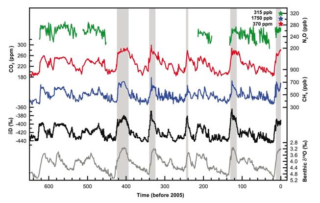
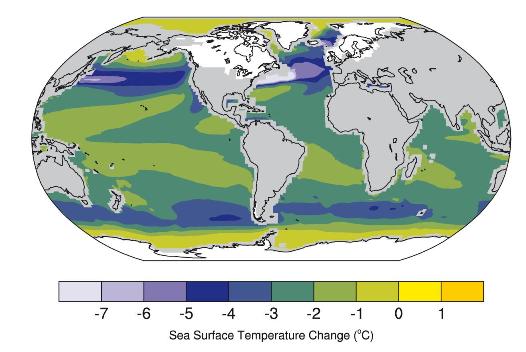
The information recorded in ice cores (Fig. 5.20) documents the alternation between long glacial periods (or Ice Ages) and relatively brief interglacials over the last 800 ka. We are currently living in the latest of these interglacials, The Holocene. The glacial period that is the best known is the latest one, which peaked around 21 ka BP and is referred to as the Last Glacial Maximum (LGM). At that time, the ice sheets covered the majority of the continents at high northern latitudes, with ice sheets as far south as 40^oN. Because of the accumulation of water in the form of ice over the continents, the sea level was lower by around 120 m, exposing new land to the surface. For instance, there was a land bridge between America and Asia across the present-day Bering Strait and another between continental Europe and Britain. The permafrost and the tundra stretched much further south than at present while rain forest was less extensive. Tropical regions were about 2-4^oC cooler than now over land and probably over the oceans as well (Fig. 5.21). The cooling was greater at high latitudes and the sea-ice extended much further in these regions. Overall, the global mean temperature is estimated to be between 4 and 7^oC lower than at present.

The orbital theory of paleoclimates assumes that the alternations of glacial and interglacial periods are mainly driven by the changes of the orbital parameters with time. In this context, the summer insolation at high northern latitudes, where the majority of the land masses are presently located, appears to be of critical importance. If it is too low, the summer will be cool and only a fraction of the snow that has fallen over land at high latitudes during winter will melt. As a consequence, snow will accumulate from year to year, and after thousands of years large ice sheets (see section 4.2.3), characteristic of the glacial periods, will form. Conversely, if summer insolation is high, all the snow on land will melt during the relatively warm summer and no ice sheet can form. Furthermore, because of the summer warming, snow melting over existing ice sheet can exceed winter accumulation leading to an ice sheet shrinking and a deglaciation. Through this feedback (and other ones, see Chapter 4), the effect of relatively small changes in insolation can be amplified, leading to the large variations observed in the glacial-interglacial cycles.

**Figure 5.20:** Variations in deuterium ( $δ$ D; black), and in the atmospheric concentrations of the greenhouse gases CO₂ (red), CH₄ (blue), and nitrous oxide (N₂O; green) derived from air trapped within ice cores from Antarctica and from recent atmospheric measurements. The grey curve is a compilation of benthic $δ$ ¹⁸O marine records from various sources. Deuterium is a proxy for local temperature (here for the temperature in Antarctica) and benthic $δ$ ¹⁸O is a proxy for global ice volume fluctuations, a high value of benthic $δ$ ¹⁸O corresponding to a low ice volume (see section 5.3.3). The stars and labels indicate the atmospheric concentrations in the year 2000. The shading indicates the last interglacial warm periods. Figure 6.3 from Jansen et al. (2007) using a modified legend, published in: Climate Change 2007: The Physical Science Basis. Contribution of Working Group I to the Fourth Assessment Report of the Intergovernmental Panel on Climate Change, Cambridge University Press, copyright IPCC 2007. Reproduced with permission. For more details on this figure as well on the sources used, see Jansen et al. (2007).

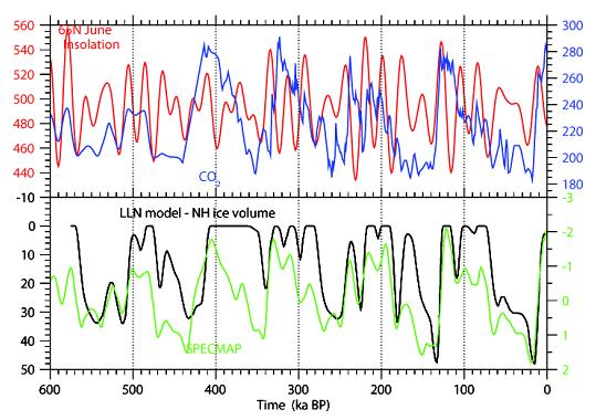
One of the most convincing arguments for the orbital theory of paleoclimate comes from the fact that the dominant frequencies of the orbital parameters are also found in many proxy records of past climate change (e.g. Fig. 5.20). This suggests a strong causal link. Another important argument comes from paleoclimate modelling. A climate model driven by changes in orbital parameters and by the observed evolution of greenhouse gases over the last 600 ka reproduced the estimated past ice volume variations quite well. If the changes in orbital parameters were not taken into account, it was not possible to simulate the pace of glacial-interglacial cycles adequately (Fig. 5.22).

**Figure 5.21:** Multi-model average change in SST between the Last Glacial Maximum climate (approximately 21 ka ago) and the pre-industrial (1750 AD) climate. Ice extent over continents is shown in white. The selected model results were compiled in the framework of the PMIP2 project (http://pmip2.lsce.ipsl.fr/). Figure 6.5 from Jansen et al. (2007) using a modified legend, published in: Climate Change 2007: The Physical Science Basis. Contribution of Working Group I to the Fourth Assessment Report of the Intergovernmental Panel on Climate Change, Cambridge University Press, copyright IPCC 2007. Reproduced with permission.

However, the link between climate change and insolation is far from being simple and linear. In particular, the correspondence between summer insolation at high latitudes and ice volume is not clear at first sight (e.g. Fig. 5.22). It appears that ice sheets can grow when summer insolation is below a particular threshold (see, for instance, the low value around 120 ka BP when the last glaciation starts). On the other hand, because of the powerful feedbacks, in particular related to the presence of ice sheets (see chapter 4), the insolation has to be much stronger to induce a deglaciation. The insolation also changes in different ways at every location and every season, making the picture more complex than that presented by a simple analysis of the summer insolation at high latitudes.

One of the most intriguing points is the predominance of strong glacial-interglacial cycles with a period of around 100 ka while this period is nearly absent from the insolation curves. The eccentricity does exhibit some dominant periods around 100 ka but it is associated with very small changes in insolation. Furthermore, until 1 million years ago, the ice volume mainly varied with a period of 40 ka, corresponding to the dominant period of the obliquity (Fig. 5.15). The importance of the 100 ka cycle over the last million years is probably related to some non-linear processes in the system. However, explaining the mechanisms involved in detail and in a convincing way is still a challenge.

**Figure 5.22:** (Top panel) The atmospheric CO₂ concentration (in ppm, blue) (as measured in the Vostok ice core over the last 414 ka (Petit et al., 1999) plus a statistical scenario for earlier dates) and the mid-month insolation value at 65^oN at the June solstice (in Wm^-2, red) according to (Berger, 1978). (Bottom panel) The Northern Hemisphere ice volume (in 10⁶ km³) simulated by the LLN 2-D climate model (Berger and Loutre, 2003) forced by insolation (Berger, 1978) and atmospheric CO₂ concentration (as in top panel) and SPECMAP curve (stacked, smoothed oxygen-isotope record in deep sea cores, Imbrie et al., 1984)